Load the data

Fist we load the data and change the date type to lubridate to facilitate working with the dates.

# Import approval polls data directly off fivethirtyeight website
approval_pollist <- read_csv('https://projects.fivethirtyeight.com/biden-approval-data/approval_polllist.csv') 

## Rows: 1597 Columns: 22

## ── Column specification ────────────────────────────────────────────────────────
## Delimiter: ","
## chr (12): president, subgroup, modeldate, startdate, enddate, pollster, grad...
## dbl  (9): samplesize, weight, influence, approve, disapprove, adjusted_appro...
## lgl  (1): tracking

## 
## ℹ Use `spec()` to retrieve the full column specification for this data.
## ℹ Specify the column types or set `show_col_types = FALSE` to quiet this message.

glimpse(approval_pollist)

## Rows: 1,597
## Columns: 22
## $ president           <chr> "Joseph R. Biden Jr.", "Joseph R. Biden Jr.", "Jos…
## $ subgroup            <chr> "All polls", "All polls", "All polls", "All polls"…
## $ modeldate           <chr> "9/10/2021", "9/10/2021", "9/10/2021", "9/10/2021"…
## $ startdate           <chr> "1/24/2021", "1/24/2021", "1/25/2021", "1/25/2021"…
## $ enddate             <chr> "1/26/2021", "1/27/2021", "1/27/2021", "1/26/2021"…
## $ pollster            <chr> "Rasmussen Reports/Pulse Opinion Research", "Maris…
## $ grade               <chr> "B", "A", "B", "B", "B", "B", "B", "B+", "B", "B",…
## $ samplesize          <dbl> 1500.00, 1313.00, 1500.00, 2200.00, 15000.00, 9211…
## $ population          <chr> "lv", "a", "lv", "a", "a", "a", "lv", "a", "a", "a…
## $ weight              <dbl> 0.32248994, 2.18932620, 0.30253321, 0.12049488, 0.…
## $ influence           <dbl> 0, 0, 0, 0, 0, 0, 0, 0, 0, 0, 0, 0, 0, 0, 0, 0, 0,…
## $ approve             <dbl> 48.00000, 49.00000, 49.00000, 58.00000, 54.00000, …
## $ disapprove          <dbl> 48.0, 35.0, 48.0, 32.0, 31.0, 31.5, 45.0, 37.0, 32…
## $ adjusted_approve    <dbl> 50.42358, 50.02881, 51.42358, 56.53645, 52.53645, …
## $ adjusted_disapprove <dbl> 41.93539, 34.63727, 41.93539, 35.37104, 34.37104, …
## $ multiversions       <chr> NA, NA, NA, NA, NA, "*", NA, NA, NA, NA, NA, NA, N…
## $ tracking            <lgl> TRUE, NA, TRUE, NA, TRUE, TRUE, TRUE, NA, TRUE, NA…
## $ url                 <chr> "https://www.rasmussenreports.com/public_content/p…
## $ poll_id             <dbl> 74261, 74320, 74268, 74346, 74277, 74292, 74290, 7…
## $ question_id         <dbl> 139433, 139558, 139483, 139653, 139497, 139518, 13…
## $ createddate         <chr> "1/27/2021", "2/1/2021", "1/28/2021", "2/5/2021", …
## $ timestamp           <chr> "18:35:08 10 Sep 2021", "18:35:08 10 Sep 2021", "1…

# Use `lubridate` to fix dates, as they are given as characters.
approval_pollist <- approval_pollist %>% 
  mutate(modeldate = lubridate::mdy(modeldate), 
         startdate = lubridate::mdy(startdate), 
          enddate = lubridate::mdy(enddate), 
          createddate = lubridate::mdy(createddate))

Create a new data frame

We calculate the average net approval rate (approve - disapprove) for each week since President Biden got into office. Then we plot the net approval, along with its 95% confidence interval. We use the ‘enddate’ as date and facet by the subgroup to see the difference between adults, voters and all polls.

The net approval rate allows us to get a feeling of how popular Biden and his policy is within the US. For different polls, the percentage of people that state they approve and the percentage of people that disapprove for the given statements is calculated. We “net” these rates and then calculate the weekly mean across the pools taken within the respective week. In addition, we calculate a 95% confidence interval for the net approval rate using the formula CI: mean +/- (t-critical * SE).

We use glimpse() to look at the new data frame we created.

# Create confidence levels
approval_margins <- approval_pollist %>%
  
  #Select enddate
  filter(!is.na(enddate)) %>%
  mutate(week=isoweek(enddate),
         net_approval_rate = adjusted_approve-adjusted_disapprove) %>% 
  
  #Group the data
  group_by(week, subgroup) %>%
  
  #Summarize data (use se formula for differences)
  summarise(
    number = n(),
    mean_net_approval_rate = mean(net_approval_rate, na.rm=TRUE),
    sd_net = sd(net_approval_rate, na.rm=TRUE),
    se = sd_net/sqrt(number),
    t_critical=qt(0.975, number- 1),
            lower_ci = mean_net_approval_rate - (t_critical*se),
            upper_ci = mean_net_approval_rate + (t_critical*se))

## `summarise()` has grouped output by 'week'. You can override using the `.groups` argument.

glimpse(approval_margins)

## Rows: 99
## Columns: 9
## Groups: week [33]
## $ week                   <dbl> 4, 4, 4, 5, 5, 5, 6, 6, 6, 7, 7, 7, 8, 8, 8, 9,…
## $ subgroup               <chr> "Adults", "All polls", "Voters", "Adults", "All…
## $ number                 <int> 9, 16, 9, 14, 23, 12, 12, 19, 9, 13, 25, 14, 13…
## $ mean_net_approval_rate <dbl> 19.17343, 16.30575, 14.95819, 17.16960, 15.9013…
## $ sd_net                 <dbl> 1.806431, 3.805121, 5.283957, 3.140905, 3.88976…
## $ se                     <dbl> 0.6021437, 0.9512803, 1.7613191, 0.8394422, 0.8…
## $ t_critical             <dbl> 2.306004, 2.131450, 2.306004, 2.160369, 2.07387…
## $ lower_ci               <dbl> 17.784883, 14.278146, 10.896579, 15.356098, 14.…
## $ upper_ci               <dbl> 20.56198, 18.33336, 19.01980, 18.98311, 17.5834…

Create the graph

We essentially plot the mean net approval rate per week. We decide to filter the subgroup=="Voters. The single data points are plotted by points and connected with a line. In addition, we add a geom_smooth() line to show the trend. More over, we plot the confidence interval using the geom_ribbon() function and fill the area it in light grey to make if visually more appealing in the graph. With the help of geom_hline() we add a horizontal line at x=0 which essentially shows the line at which approval rate would equal disapproval rate.

#Create the graph
approval_margins %>% 
  filter(subgroup == "Voters") %>%
  ggplot(aes(x=week, y= mean_net_approval_rate)) +
  
  #Set colors 
  geom_point(color="chocolate2", size=1.5) +
  geom_line(color="chocolate2") +
  
  #Add fill between lines
  geom_ribbon(aes(ymin=lower_ci, ymax=upper_ci),
              color="chocolate2", 
              fill="grey87", 
              linetype=1, 
              alpha=0.5, 
              size=0.3) +
  
  facet_wrap(~subgroup) +
  
  #Change limits, theme, scale, facet wrap and add fitted line 
  ylim(c(-15,50)) +
  theme_bw() +
  scale_x_continuous(breaks=seq(0, 35, 13))+
  scale_y_continuous(breaks=seq(-15, 10, 2.5))+
  geom_smooth(se=FALSE) +
  
  #Add horizontal line 
  geom_hline(yintercept=0, 
             linetype="solid",
             color = "chocolate2", 
             size=2) +
  
  #Add labels 
  labs( title="Estimating Approval Margins (approve-disapprove) for Joe Biden",
        subtitle = "Weekly average of all polls",
        x = "Week of the year",
        y = "Average Approval Margin (Approve - Disapprove)") +
  NULL

## Scale for 'y' is already present. Adding another scale for 'y', which will
## replace the existing scale.

## `geom_smooth()` using method = 'loess' and formula 'y ~ x'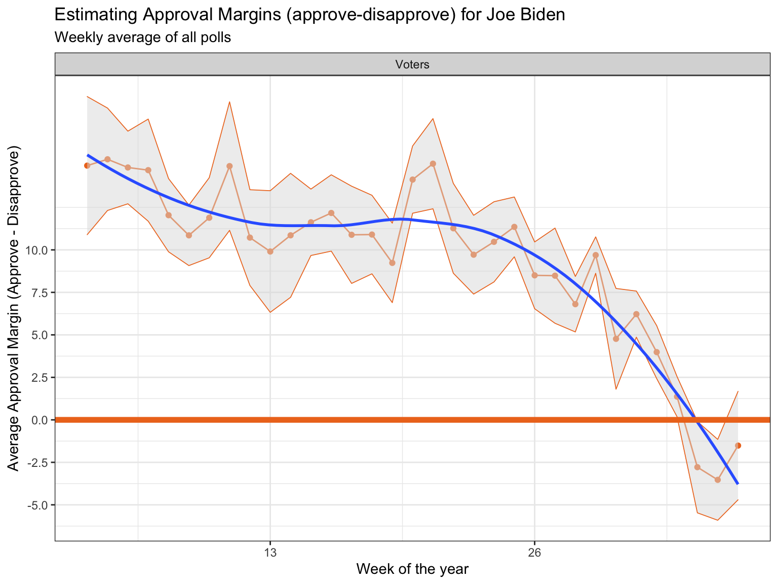

Analysis

Looking at the confidence interval, we can see that its size greatly differ between the different weeks. One of the reasons for this is that the sample set size differ. For example, the sample size of week 4 is much smaller than that of week 25 which is why the standard error is relatively higher in week 4. This leads to larger confidence intervals in week 4 compared to week 25. As far as the data across the weeks is concerned, the approval ratings for Joe Biden have decreases significantly over the weeks. While they started reasonably high, they have no gone into slight negative net approval. However, as the confidence interval shows, there is some uncertainty related to these polls as they are derived only from a small sample in comparison to the entire population.