Germany election 2021 forecast

Calculate 2-week moving average of opinion polls for the 2021 German elections
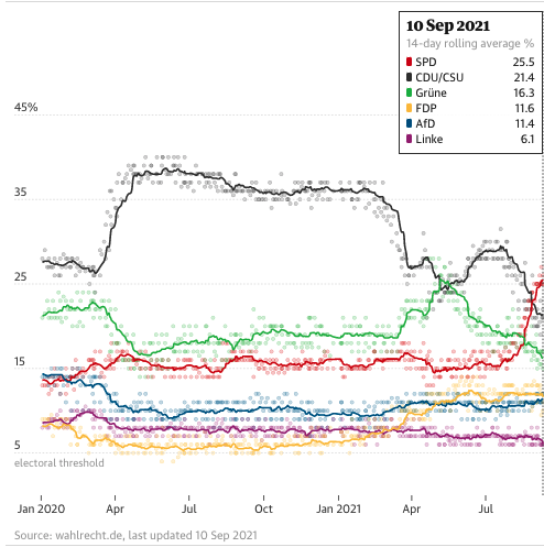
The Guardian newspaper has an election poll tracker for the upcoming German election. The list of the opinion polls since Jan 2021 can be found at Wikipedia. Here we will reproduce the graph with the following code. As a reference, please see the picture from The Guardian below that is replicated with the code. However, we choose to only plot the values for 2021. Essentially, we look at all voting polls from 2021 and calculate a 14-day moving average which we then plot. We do this to see the changes in voting forecasts leading up to the German federal election in September 2021.
Graph we will replicate:
Load the data
First we load the data and adjust the date type to lubridate so that we can work with it.
url <- "https://en.wikipedia.org/wiki/Opinion_polling_for_the_2021_German_federal_election"

# get tables that exist on wikipedia page
tables <- url %>%
  read_html() %>%
  html_nodes(css="table")


# parse HTML tables into a dataframe called polls
# Use purr::map() to create a list of all tables in URL
polls <- map(tables, . %>%
             html_table(fill=TRUE)%>%
             janitor::clean_names())


# list of opinion polls
# the first table on the page contains the list of all opinions polls
german_election_polls <- polls[[1]] %>%

  # drop the first row, as it contains again the variable names and last row that contains 2017 results
  slice(2:(n()-1)) %>%
  mutate(

         # polls are shown to run from-to, e.g. 9-13 Aug 2021. We keep the last date, 13 Aug here, as the poll date
         # and we extract it by picking the last 11 characters from that field
         end_date = str_sub(fieldwork_date, -11),

         # end_date is still a string, so we convert it into a date object using lubridate::dmy()
         end_date = dmy(end_date),

         # we also get the month and week number from the date, if we want to do analysis by month- week, etc.
         month = month(end_date),
         week = isoweek(end_date))
Create and mutate the dataframe
Then we create a dataframe with the columns of data we are actually interested in for the analysis. In addition we mutate the dataframe so that all information we need to create the graph is available. For example, we take the sample size of every poll and multiply it with the voting fraction to get the total number of voters for a specific party by the respective poll. Then, in the next step, we can add up multiple polls by adding the voters across poll of a specific party and dividing it by total number of asked people for the sum of poll taken. This is important as we calculate the 14-day moving average poll prediction for the individual parties. We cannot simply average the percentages by parties reported by the dataset, but need to recaclulate given that the different polls had different sample sizes.
german_polls <- german_election_polls %>%

  #Select parties data we need
  select(polling_firm, end_date, samplesize, union, spd, af_d, fdp, linke, grune) %>%

  #Eliminate "," from sample size so that we can change it to numeric
  mutate(samplesize= gsub("," , "" , samplesize)) %>%

  #Change samplesize from chr to numeric
  mutate(samplesize=as.numeric(samplesize)) %>%

  #Calculate actual votes per party
  mutate(union_votes=samplesize*(union/100),
         spd_votes=samplesize*(spd/100),
         af_d_votes=samplesize*(af_d/100),
         fdp_votes=samplesize*(fdp/100),
         linke_votes=samplesize*(linke/100),
         grune_votes=samplesize*(grune/100)) %>%

  #Calculate 14 day moving average of samplesize across different surveys
  mutate(samplesizem = movavg(samplesize, 14, "s"),

        #Calculate moving average % per party
         unionm = (movavg(union_votes, 14, "s")/samplesizem*100),
         spdm = (movavg(spd_votes, 14, "s")/samplesizem*100),
         af_dm = (movavg(af_d_votes, 14, "s")/samplesizem*100),
         fdpm = (movavg(fdp_votes, 14, "s")/samplesizem*100),
         linkem = (movavg(linke_votes, 14, "s")/samplesizem*100),
         grunem = (movavg(grune_votes, 14, "s")/samplesizem*100),
         )

glimpse(german_polls)
## Rows: 229
## Columns: 22
## $ polling_firm <chr> "INSA", "GMS", "Forsa", "INSA", "Forschungsgruppe Wahlen"…
## $ end_date <date> 2021-09-13, 2021-09-13, 2021-09-13, 2021-09-10, 2021-09-…
## $ samplesize <dbl> 2062, 1003, 2501, 1152, 1281, 1901, 1208, 10082, 1700, 12…
## $ union <dbl> 20.5, 23.0, 21.0, 20.0, 22.0, 21.0, 19.0, 23.0, 21.0, 25.…
## $ spd <dbl> 26, 25, 25, 26, 25, 25, 28, 25, 26, 27, 26, 25, 25, 25, 2…
## $ af_d <dbl> 11.5, 11.0, 11.0, 11.0, 11.0, 12.0, 11.0, 11.0, 12.0, 11.…
## $ fdp <dbl> 12.5, 13.0, 11.0, 13.0, 11.0, 12.0, 12.0, 11.0, 10.0, 9.5…
## $ linke <dbl> 6.5, 6.0, 6.0, 6.0, 6.0, 6.0, 6.0, 6.0, 6.0, 6.0, 6.5, 6.…
## $ grune <dbl> 15.0, 16.0, 17.0, 15.0, 17.0, 17.0, 14.0, 17.0, 15.0, 15.…
## $ union_votes <dbl> 423, 231, 525, 230, 282, 399, 230, 2319, 357, 314, 421, 2…
## $ spd_votes <dbl> 536, 251, 625, 300, 320, 475, 338, 2520, 442, 340, 534, 2…
## $ af_d_votes <dbl> 237, 110, 275, 127, 141, 228, 133, 1109, 204, 138, 226, 1…
## $ fdp_votes <dbl> 258, 130, 275, 150, 141, 228, 145, 1109, 170, 120, 256, 1…
## $ linke_votes <dbl> 134.0, 60.2, 150.1, 69.1, 76.9, 114.1, 72.5, 604.9, 102.0…
## $ grune_votes <dbl> 309, 160, 425, 173, 218, 323, 169, 1714, 255, 195, 318, 1…
## $ samplesizem <dbl> 2062, 1532, 1855, 1680, 1600, 1650, 1587, 2649, 2543, 241…
## $ unionm <dbl> 20.5, 21.3, 21.2, 21.0, 21.1, 21.1, 20.9, 21.9, 21.8, 22.…
## $ spdm <dbl> 26.0, 25.7, 25.4, 25.5, 25.4, 25.3, 25.6, 25.3, 25.4, 25.…
## $ af_dm <dbl> 11.5, 11.3, 11.2, 11.2, 11.1, 11.3, 11.3, 11.1, 11.2, 11.…
## $ fdpm <dbl> 12.5, 12.7, 11.9, 12.1, 11.9, 11.9, 11.9, 11.5, 11.4, 11.…
## $ linkem <dbl> 6.50, 6.34, 6.19, 6.15, 6.13, 6.10, 6.09, 6.05, 6.05, 6.0…
## $ grunem <dbl> 15.0, 15.3, 16.1, 15.9, 16.1, 16.2, 16.0, 16.5, 16.4, 16.…#create legend numbers following each party
union_rate <- german_polls %>% filter(end_date == end_date[length(end_date)]) %>% select(union)
spd_rate <- german_polls %>% filter(end_date == end_date[length(end_date)]) %>% select(spd)
af_d_rate <- german_polls %>% filter(end_date == end_date[length(end_date)]) %>% select(af_d)
fdp_rate <- german_polls %>% filter(end_date == end_date[length(end_date)]) %>% select(fdp)
linke_rate <- german_polls %>% filter(end_date == end_date[length(end_date)]) %>% select(linke)
grune_rate <- german_polls %>% filter(end_date == end_date[length(end_date)]) %>% select(grune)
#paste the text and number together
union_rate <- paste("Union ", union_rate[1,1])
spd_rate <- paste("SPD ", spd_rate[1,1])
af_d_rate <- paste("AfD ", af_d_rate[1,1])
fdp_rate <- paste("FDP ", fdp_rate[1,1])
linke_rate <- paste("Linke ", linke_rate[1,1])
grune_rate <- paste("Grune ", grune_rate[1,1])Create the final graph
Finally, we actually plot the graph using the mutated data frame from before. We want to plot the all poll individually with points. In addition, we add a line with the 14-day moving average across the different polls taken within that time period. The 14-day moving average essentially smoothens out some of the volatility and makes it easier to see trends across the different polls.
We also ensure that the lines and points have the correct color depending on the party, adjust the axis to make it visually more appealing and label the graph appropriately.
#Create the table
german_polls %>%
  select(end_date, union, spd, af_d, fdp, linke, grune, unionm, spdm, af_dm, fdpm, linkem, grunem) %>%
  ggplot() +

  #Add color depending on party
  geom_point(aes(x=end_date,y=union, color="black"), alpha=0.2) +
  geom_line(aes(x=end_date,y=unionm), color="black") +
  geom_point(aes(x=end_date,y=spd, color="red"), alpha=0.2) +
  geom_line(aes(x=end_date,y=spdm), color="red") +
  geom_point(aes(x=end_date,y=af_d, color="blue"), alpha=0.2) +
  geom_line(aes(x=end_date,y=af_dm), color="blue") +
  geom_point(aes(x=end_date,y=grune, color="green"), alpha=0.2) +
  geom_line(aes(x=end_date,y=grunem), color="green") +
  geom_point(aes(x=end_date,y=fdp, color="yellow"), alpha=0.2) +
  geom_line(aes(x=end_date,y=fdpm), color="yellow") +
  geom_point(aes(x=end_date,y=linke, color="purple"), alpha=0.2) +
  geom_line(aes(x=end_date,y=linkem), color="purple") +

  #Add horizontal dashed lines
  geom_hline(yintercept=5, linetype="dashed",color = "grey", size=0.5) +
  geom_hline(yintercept=15, linetype="dashed",color = "grey", size=0.5) +
  geom_hline(yintercept=25, linetype="dashed",color = "grey", size=0.5) +
  geom_hline(yintercept=35, linetype="dashed",color = "grey", size=0.5) +
  geom_hline(yintercept=45, linetype="dashed",color = "grey", size=0.5) +

  #Add text
  geom_text(aes(end_date[length(end_date)],5, label= "  electoral threshold", color = "grey", vjust=1, hjust=0.3), size=3) +

  #Set colors of legend
  scale_color_identity(name= "10 Sep 2021", breaks=c("black", "red", "blue", "green", "yellow", "purple"),
                       labels=  c(union_rate, spd_rate, af_d_rate, grune_rate, fdp_rate, linke_rate),
                       guide = "legend") +

  theme_bw() +

  theme(legend.background = element_rect(color = "black"), panel.grid = element_blank(),
        legend.position = c(0.925,0.756),
        legend.title = element_text(size = 10, face = "bold"),
        legend.text = element_text(size = 8), legend.key.size = unit(1, "lines"),
        legend.spacing.y = unit(0.01, "cm"),
        plot.caption = element_text(hjust = 0)) +

   #Adjust y axis
  scale_y_continuous(breaks = c(5, 15, 25, 35, 45),
                     labels = c("5", "15", "25", "35", "45%"),
                     limits = c(0, 70)) +

  #Adjust x axis
  scale_x_continuous(breaks = c(german_election_polls$end_date[214],
                                german_election_polls$end_date[151],
                                german_election_polls$end_date[67]),
                     labels = c("Jan 2021", "Apr", "Jul")) +

  #Label the graph
  labs(caption = "Source: wahlrecht.de, last updated 10 Sep 2021",
  title="German election poll tracker: who will be the next chancellor?",
  subtitle = "Find out who is leading the polling to succeed Angela Merkel as chancellor of Germany",
  x = "",
  y = "") +
  NULL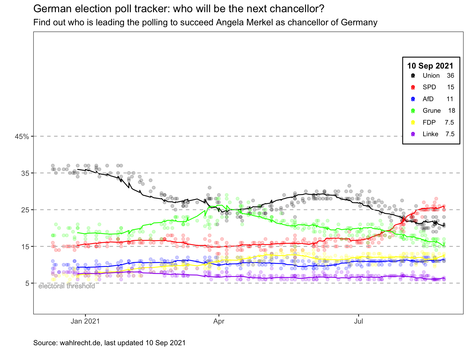
Observations
We can see that at the beginning of 2021, the Union (also known as CDU), was by far the most popular party across the polls. However, with time, their poll rates decreased significantly. The SPD, led by Chancellor candidate Olaf Scholz, however, experienced an opposite trend. Especially from July to August, SPD gained significant share of the polls, which is an indication for popularity. Hence, as of the beginning of September, is not yet visible who will succeed Angela Merkel as the Chancellor of Germany.